Introduction

Modelling species, habitats and their relationships to environmental pressures is complex, as cause and effects are intertwined and impacts are often mitigated through a set of attributes that cannot easily be modelled using standard techniques. An example is given in the figure below. This conceptual model was developed at a meeting organised with Fisheries experts. The participants produced a model of trout habitat (in blue) and its relationship to environmental pressures (in red).

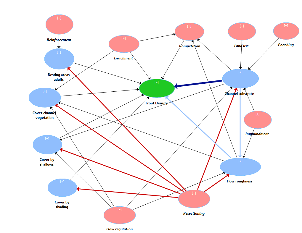
Most environmental attributes had a direct link to fish density, but they also influenced each other adding to the model complexity. For example, channel substrate had both a direct (thick blue arrow) and indirect (thin light blue arrow) influence on trout density through its effect on flow roughness. Channel resectioning had no direct effect on fish density; instead, its influence was mediated through its impact on other habitat attributes such as channel substrate, flow velocity patterns, the presence of cover and resting areas (red arrows).

Traditional statistical techniques such as linear regression mainly model direct impacts of uncorrelated variables. Indirect effects are difficult to model and the presence of correlations between explanatory variables may lead to biased coefficient estimates and incorrect model interpretation.

Structural Equation Modelling (SEM) is an extension of linear regression that enables the modelling of complex relationships between interrelated (and thus correlated) variables.  The method is simple, intuitive and requires basic statistical and modelling knowledge.  It can be implemented using simple software with user-friendly graphical interfaces.  Because SEM models account for direct and indirect impacts and can cope with correlated variables, it is one of the few modelling techniques that can be used to model causal relationships.

In this paper, we show how SEM can be used to model pressures and impact on hydromorphology and species using causal models derived by experts and validated using monitoring data (Naura et al. 2011). The method was applied to modelling fish habitat (Naura 2014) and it has since been applied to biological metrics (Surridge et al 2014).

Methods summary

In the example above, we developed a model of trout habitat using expert opinion that we tested using environmental data from existing monitoring programmes. The model was implemented with Smart-PLS, a bespoke SEM statistical software with a friendly user interface (https://www.smartpls.com/).

The data were derived from water quality, fisheries and River Habitat Survey databases and from hydrological models.  The data points were paired using a Geographical Information System and more than 2,500 paired sites were used for the analyses.  Each habitat feature and environmental pressure identified by experts was associated with relevant attributes from existing monitoring databases. For example, channel substrate was characterised using data from the River Habitat Survey describing the occurrence of channel substrate types at 10 transects.

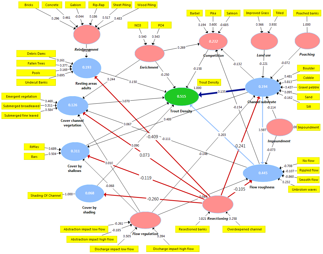
In SEM, it is possible to use more than one attribute to characterise a habitat feature or dimension of interest. These dimensions are called Latent Variables (LVs) and are displayed as coloured oval shapes.  In the example above, the Latent Variables describing ‘channel substrate’ and ‘flow roughness’ were defined as combinations of channel substrate and flow-type categories. ‘Resting areas for adults’ was defined according to the presence of various habitat features such as debris dams, fallen trees, pools or undercut banks that provide cover for fish.  SEM uses an optimisation process to create an index score for each LV using linear regression. The method is similar to Principal Component Analysis. Once defined, LVs are regressed against each other to produce the final model outputs (see figure below).

Each causal arrow is associated with a standard coefficient representing impact on a scale of -1 (high negative impact) to +1 (high positive impact). The numbers displayed in the LVs oval shapes represent R² values, i.e. the amount of variability explained by the LVs predicting them. In our case, 51.5% of trout density variability could be explained by the model.

The outputs can be best summarised in a table (see below) representing all impacts from each habitat feature and pressure on each other and on trout density, taking account of direct and indirect effects.

Rows relating to environmental pressures were shaded in grey.  Substrate, flow roughness and resting areas for adults had the highest positive impact on trout density (see data in column with thick black border). Enrichment by phosphates and nitrates, resectioning and the presence of competitors had the highest negative impact on fish.  The way the impact of pressures is mediated is also described in the table.  Channel resectioning strongly influenced the presence of resting areas, cover, flow roughness and channel substrate with impact coefficients varying between -0.2 to -0.4. In comparison, bank reinforcement had little overall impact on fish density although it had some influence on the presence of resting areas for adult trout. Thus, using the graph and table we can quantify the impacts of pressures on hydromorphology and species at reach scale, and identify potential causes of failure in ecological status as well as causal pathways.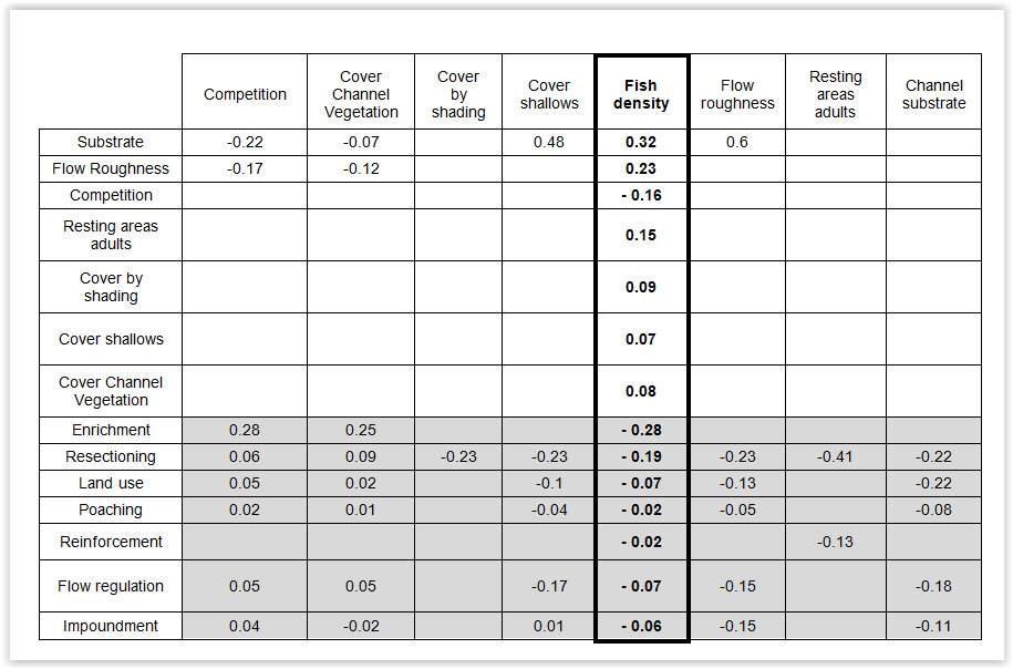

Implementation

The model was applied to all existing RHS sites and a visual interface in ToolHab was produced to represent the model outputs and enable the identification of potential pressures and impacts by catchment officers (figure below).  The middle column contains trout habitat features.  Boxes are coloured according to their overall impact on fish densities (blue = high positive impact, red = low positive impact).  The arrows show links of causality between features and trout.  The thickness of the arrows represents the strength of the impact and the colour its direction (blue = positive impact, orange = negative impact).  In the left-hand column are pressures on hydromorphology and fish.  The colour of the boxes represents the level of impact each pressure has on total fish densities.  The arrows represent the impact of pressures on individual habitat attributes or fish density.

Conclusion

The approach demonstrates how expert opinion and data from existing monitoring programs can be used in combination to produce causal models linking pressures, hydromorphological dimensions and species. The models can then be turned into graphical interfaces enabling the diagnostic and assessment of potential causes of failure to ecological status targets and the identification of relevant management options. SEM is a simple but powerful modelling technique that is intuitive, visual and easy to implement and apply.

Acknowledgements

This work was carried out as part of an EPSRC funded fellowship at the University of Southampton (Faculty of Engineering and the Environment) as well as funding from the School of Geography, the Environment Agency and the Scottish Environment Protection Agency .

References

Naura, M. (2014) Decision Support Systems. Factors affecting their design and implementation within organisations.  Lessons from two case studies. Berlin. Lambert Academic Publishing. (link to website: http://tinyurl.com/mal5pat).

Naura, M., Sear, D., Alvarez, M., Penas, F., Fernandez, D. & Barquin, J. (2011) Integrating monitoring, expert knowledge and habitat management within conservation organisations for the delivery of the water framework directive: A proposed approach. Limnetica, 30, 427-446.

Surridge, B.W.J., Bizzi, S. & Castelletti, A. (2014) A framework for coupling explanation and prediction in hydroecological modelling. 61, 274-286.